This report is based on two separate surveys conducted on Pew Research Center’s American Trends Panel. The ATP is a nationally representative panel of randomly selected U.S. adults recruited from landline and cellphone random-digit-dial surveys. Panelists participate via monthly self-administered web surveys. Panelists who do not have internet access are provided with a tablet and wireless internet connection.
The first of the two surveys analyzed in this report, which included an open-ended question about what makes life meaningful and fulfilling, was conducted in September 2017. Details about the survey and the methods used to code the open-ended responses are provided below.
The second survey, which included closed-ended questions about what makes life meaningful and fulfilling, was conducted in December 2017. The overall results of the December 2017 survey have been previously released (however, the analysis reported here is new), and methodological details, including question wording, are available in Pew Research Center’s report “The Religious Typology.”
Survey data collection – September 2017 survey
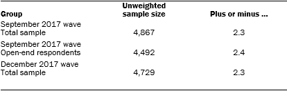
The open-ended question discussed in this report was included in an ATP survey conducted Sept. 14 to 28, 2017, among 4,867 respondents, including 4,492 respondents who provided a response to the open-ended question. The analyses reported here are based on the subset of participants who completed the open-ended question; the overall margin of sampling error for these 4,492 respondents is plus or minus 2.4 percentage points.5
Members of the American Trends Panel were recruited from several large, national landline and cellphone random-digit-dial surveys conducted in English and Spanish. At the end of each survey, respondents were invited to join the panel. The first group of panelists was recruited from the 2014 Political Polarization and Typology Survey, conducted Jan. 23 to March 16, 2014. Of the 10,013 adults interviewed, 9,809 were invited to take part in the panel and a total of 5,338 agreed to participate.6 The second group of panelists was recruited from the 2015 Pew Research Center Survey on Government, conducted Aug. 27 to Oct. 4, 2015. Of the 6,004 adults interviewed, all were invited to join the panel, and 2,976 agreed to participate.7 The third group of panelists was recruited from a survey conducted April 25 to June 4, 2017. Of the 5,012 adults interviewed in the survey or pretest, 3,905 were invited to take part in the panel, and a total of 1,628 agreed to participate.8
The ATP data were weighted in a multistep process that begins with a base weight, which incorporates the respondents’ original survey selection probability and the fact that in 2014 some respondents were subsampled for invitation to the panel. Next, an adjustment was made for the fact that the propensity to join the panel and remain an active panelist varied across different groups in the sample. The final step in the weighting uses an iterative technique that aligns the sample to population benchmarks on a number of dimensions. Gender, age, education, race, Hispanic origin and region parameters come from the U.S. Census Bureau’s 2016 American Community Survey. The county-level population density parameter (deciles) comes from the 2010 U.S. decennial census. The telephone service benchmark comes from the July-December 2016 National Health Interview Survey and is projected to 2017. The volunteerism benchmark comes from the 2015 Current Population Survey Volunteer Supplement. The party affiliation benchmark is the average of the three most recent Pew Research Center general public telephone surveys. The internet access benchmark comes from the 2017 ATP Panel Refresh Survey. Respondents who did not previously have internet access are treated as not having internet access for weighting purposes. Sampling errors and statistical tests of significance take into account the effect of weighting. Interviews are conducted in both English and Spanish, but the Hispanic sample in the American Trends Panel is predominantly U.S. born and English speaking.
The September 2017 wave had a response rate of 73% (4,867 responses among 6,696 individuals in the panel). Taking account of the combined, weighted response rate for the recruitment surveys (10.0%) and attrition of panel members who were removed at their request or for inactivity, the cumulative response rate for the wave is 2.5%.9
Identifying themes within open-ended responses
In the first survey, researchers asked the following question:
We’re interested in exploring what it means to live a satisfying life. Please take a moment to reflect on your life and what makes it feel worthwhile – then answer the question below as thoughtfully as you can.
What about your life do you currently find meaningful, fulfilling, or satisfying? What keeps you going, and why?
To avoid the risk of priming bias, the question was placed near the beginning of the survey, immediately following three introductory “ladder of life” questions that asked respondents to rate their lives on a scale of 1-10 in the past, present and future. Respondents wrote 41 words on average in answering the question about what makes life meaningful, fulfilling or satisfying. The shortest responses consisted of just a single word (66 responses in total; “family,” “work,” “God,” etc.) and the longest response totaled 939 words. Half of the panelists also received a randomly assigned expanded prompt that explicitly asked for detail – “Please give as much detail as you can” – those respondents wrote an additional 12 words on average.
Each response was coded as to whether it contained mentions of each of 30 topics or themes.10 Decisions about which themes to code for and which keywords to use as indicators were informed by a topic model. Responses were coded as having mentioned a topic if the response included any of several keywords determined by researchers to be indicators of the topic in question, or, in one case, if the model predicted that a response mentioned the topic. For instance, responses were coded as having mentioned travel if they included any of the following words or phrases: “travel,” “traveling,” “vacation,” “trip,” “adventure,” “visiting,” “new place,” “explore world” and “overseas.” Responses that do not include any of those words are coded as having not mentioned travel. (A complete list of the 30 themes coded in this analysis is provided in the appendix, along with full details about the keywords used as indictors for each topic.)
The remainder of this section provides additional details about how the text responses were processed and how the 30 topics coded in the analysis were decided upon.
Text processing
Prior to analysis, responses were cleaned using a series of standard text-processing steps: responses were broken down into whitespace-separated tokens, lowercased and lemmatized (reduced to their root form); punctuation was also removed. A series of 434 stop words were also removed: 316 common English filler words that hold little meaning (such as “the,” “a,” “and,” “but”), 24 words and abbreviations related to months (“June,” “July”), and 94 words from a custom list that was developed iteratively, mainly comprised of words contained in the survey prompt (which respondents sometimes reiterated; “satisfying,” “meaningful,” “fulfilling”) and other words that were uniquely common in the survey responses but not useful for analysis (“personally,” “especially,” “ultimately”). The following example shows how these steps affect the text:
Before: “I finally have a child. I have a wonderful husband and a job that allows me to have flexibility.” After: “finally child wonderful husband job allows flexibility”
Responses were then broken down into “bags of words,” a common approach in natural language processing that involves converting the cleaned text of responses into sets of words and phrases. Researchers chose to represent responses in terms of single words, two-word phrases (bigrams), and three-word phrases (trigrams). For example:
Before: “finally child wonderful husband job allows flexibility” After: “finally,” “child,” “wonderful,” “husband,” “job,” “allows,” “flexibility,” “finally child,” “child wonderful,” “wonderful husband,” “husband job,” “job allows,” “allows flexibility,” “finally child wonderful,” “child wonderful husband,” “wonderful husband job,” “husband job allows,” “job allows flexibility”
In addition to removing stop words, researchers also filtered out words and phrases that were found in fewer than five different responses and removed those that were found in more than 90% of all responses (extremely frequent words often do not capture meaningful variation).
At the end of this process, the remaining vocabulary consisted of 1,603 unigrams, 1,082 bigrams and 111 trigrams, and each document was flagged as containing each word or phrase, or not, using binary variables. These 2,796 flag variables were then passed into topic models, which attempted to identify clusters of words.
Developing codable topics and identifying associated keywords through topic models
After processing the text, researchers entered the responses into a variety of computational topic models.11 Two different semi-supervised topic models – a granular one with 110 topics, and smaller one with 55 topics – initially returned 165 possible themes, which at this stage were simply sets of words that tended to appear together within responses.12 Researchers reviewed a sample of responses containing each of the sets of words, and then iteratively refined the models by adding anchor words to direct the models toward more conceptually coherent themes, with the goal of being able to assign each theme a clear definition. Researchers also identified spurious words in the topics that actually referred to a different concept than what the topic was intended to measure, and flagged these as irrelevant words to exclude from the topics in subsequent iterations of the model.
To provide a concrete example, one topic that emerged during exploratory topic modeling included the words “grandchild,” “grand,” “child grandchild,” “grand child,” “child” and “Florida.” While these words were correlated with one another in the dataset, researchers determined that this topic’s main theme was grandchildren, and the word “Florida” was related to a different concept (those who mentioned living in Florida were also especially likely to mention grandchildren). Accordingly, subsequent iterations of the topic model were instructed to assign “Florida” to a different topic.
Researchers repeated these processes several times, and ultimately settled on a finite set of potentially codable themes or topics. For each of these potentially codable topics, the research team developed a codebook consisting of a specific definition for what the topic represented, and additional guidelines for which types of responses qualified and which did not. Next, researchers drew a random sample of 100 responses for each of the potentially codable topics. For each sample, researchers used the codebook to classify whether each response mentioned the topic or not, according to its definition.
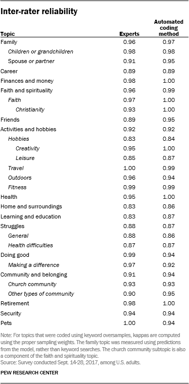
Two in-house coders completed each sample, with the goal of producing acceptable inter-rater reliability, which was defined as achieving 95% confidence that Cohen’s kappa (a common reliability measure) was above 0.70 (a common threshold for good agreement). Whether the codes for a topic’s sample managed to reach this threshold depended on two things: the reliability between the two coders in their coding of the sample of 100 documents, and the prevalence of the topic in the sample (that is, how often it appeared). Because of the small sample sizes and resulting uncertainty, the actual kappa values required to reach the 95% confidence cutoff were much higher than 0.70. Researchers were able to reach this threshold for many of the topics identified as potentially codable, identified some as clearly not reliably codable, and found that several topics showed acceptable reliability but failed to meet the 95% confidence threshold because they were relatively rare and the sample size was not large enough.
For the latter set of topics (those that showed acceptable reliability but failed to meet the 95% confidence threshold), researchers had to code additional documents to meet the confidence threshold. For some of these topics, researchers were able to accomplish this by expanding the existing random samples. However, this was not a viable approach for a few topics that appeared less frequently; for these, researchers used a technique called keyword oversampling to draw new samples. Rather than code another, much larger random sample for topics that were present in only a small fraction of documents, the lists of anchor words were used to draw new samples that were disproportionately comprised of documents that contained each of the topics being investigated: 50% with and 50% without. Based on the assumption that roughly half of the documents in these samples would contain the actual themes researchers were attempting to code, the expected Cohen’s kappa (based on the initial random samples for each topic) was used to estimate the number of documents that would be required for each of the new samples in order to successfully verify that reliability was above 0.70.13
After coding these samples and computing Cohen’s kappa values using sampling weights (which penalized false negatives that did not contain the oversampled anchor words), all of these topics were determined to be codable. While the topic models produced predictions about which responses mentioned particular topics, they also included a list of anchor words, consisting of the most prominent words in each topic, as well as additional words that were related to each topic and added manually by researchers. These keywords were used as an alternative way to measure whether responses mentioned a topic: By formatting the anchor words as keyword matching patterns (known as regular expressions), researchers could search through the text and identify any responses that used one or more of a topic’s keywords.
Next, researchers resolved their own disagreements for each of the topic samples proven to be reliably codable, resulting in a human-produced ground truth for each category. This baseline estimate of which responses mentioned particular topics could be compared against both the keyword-matching pattern for each topic and the predictions from the topic model. For almost all of the codable topics, researchers were able to successfully verify that an automated topic-modeling method could reliably emulate human coders. However, the topic model only outperformed keyword matching for one of the codable topics; for most topics, simply searching responses for any of the keywords among each topic’s most prominent words proved to have higher reliability. Accordingly, researchers decided to use keyword searches as the primary method of topic identification, rather than the anchored models. Only one topic (general references to family) was measured using the topic model predictions; all others were measured using anchor word regular expressions.
At this point, researchers re-examined more than a dozen topics that had been set aside during earlier coding due to poor reliability. Researchers refined the keywords for each of these topics and created a new codebook definition for each. Next, they drew keyword-weighted samples (rather than random samples), each sized according to prevalence of the topic during prior coding attempts. After coding, resolving disagreements and comparing the researcher benchmarks against the automated pattern matching, acceptable kappa values were achieved for most of these re-examined topics (for both human coder and human-pattern agreement).
Finally, researchers reviewed 200 random documents alongside the (now nearly final) topic codes and conducted an open-coding exercise intended to identify any additional prominent topics that were not being captured by the existing topics. Through this process, researchers identified one additional theme (helping others) that was added to the list of topics being coded.
This process initially resulted in 38 codable topics, some of which consisted entirely of component subtopics. Two of these 38 were used to capture references to family in general and faith and spirituality in general. These two were not analyzed on their own and another six were set aside because they did not appear frequently in the data; the remaining 30 topics were used in the final analysis.14
Six topics (family, faith and spirituality, activities and hobbies, struggles, doing good, and community and belonging) have hierarchical relationships with other topics. For example, the activities and hobbies topic contains the anchor words for its six subtopics: hobbies, creativity, leisure, travel, outdoors and fitness. Similarly, responses are coded as having mentioned the topic family if they mention spouses and romantic partners or children and grandchildren (each of which are also coded separately), or if they make general mention of family or relatives other than spouses, children and grandchildren.
The 30 topics researchers examine in the analysis are shown below, along with indicators of the inter-rater reliability achieved in the coding of each topic.
The complete list of topics appears in Appendix A, along with each topic’s codebook definition and the final list of anchor words. It is important to note that these word lists and interpretations were developed specifically for use on this particular dataset (i.e. the unique frequency of and context in which these words were used in this particular set of survey responses) and these keywords may not produce reliable results for other text datasets.
Regression analysis
Researchers tested all the demographic correlates of having mentioned each topic using survey-weighted logistic regressions that included each of the following factors:
- Race/ethnicity
- Religion
- Education
- Age
- Income
- Political ideology (5-point scale)
- Ideological extremity (moderate vs. very liberal or very conservative)
- Gender
- Self-reported urbanicity of their place of residence (urban, rural, suburban)
- U.S. geographic region (West, Midwest, Northeast, South)
- Marital status
- Whether the respondent has children
- Survey language (English or Spanish)
- Logged word count15
By including the last variable – word count – researchers were able to identify demographic differences in the rates that certain topics were mentioned, holding constant the amount of text that a particular respondent wrote. Because of outliers, word count was transformed using a logarithmic scale to more closely approximate a normal distribution. In this report, all discussion of the open-ended responses take into account the results of these regression models. That is to say, groups are not described in this report as being different than one another (in their propensity to mention a given topic) unless the differences are statistically significant in the regression model.
The dependent variable in each of these models was whether a particular topic was mentioned by respondents. Each model was also estimated multiple times, alternating the base category of each categorical independent variable in the model across every possible value, to ensure that results were not conditional on the selection of any particular base category.
Robustness and sensitivity analysis
Because the analysis examined small demographic groups and topics that were mentioned infrequently, researchers attempted to address the possibility that observed differences were due to classification error. This kind of error emerges when keywords for a particular topic appear in responses that do not actually discuss the topic of interest. As an example, sometimes individuals mentioned that they enjoyed “working out,” which would incorrectly be classified as a reference to a job, because it contained the keyword “working.” For some of the smaller demographic groups in the sample, even a 5% or 10% false positive rate could produce misleading results.
To assess this risk, researchers examined all relationships of interest using a series of multiple regression models. In each iteration of these models, researchers introduced measurement error into the dataset and checked whether the results were comparable. All results are robust to this test, which is described in more detail below.
To create an estimate of measurement error for these tests, researchers used the results of the inter-rater reliability analysis to compute the precision (rate of false positives) and recall (rate of false negatives) for each topic. This allowed them to measure exactly how often certain keyword lists produced incorrect results. With these rates in hand, researchers conducted a sensitivity analysis in which they repeatedly reversed the topic classifications for different subsets of responses. Then, after estimating a series of regression models, they assessed the statistical significance of particular demographic differences.
Researchers used the precision score for each topic to calculate the number of responses in the full dataset that the topic flagged that could be false positives, and they used the recall score to calculate the number of responses the topic may have missed. Researchers then created 100 simulated datasets meant to approximate this measurement error. In other words, in these simulated datasets, researchers switched positive responses to negative ones, and negative ones to positive, according to the false positive or negative rates observed in the comparison with human coders.
For example, if a topic had a precision score of 94%, 6% of the positive cases it flagged could be incorrect. And, if the same topic had a 92% recall, 8% of the true positive cases could have been incorrectly flagged as negatives. By taking 6% of the positive cases for a given topic and turning them negative (and vice versa for 8% of the negative cases) and then repeating this process 100 times, researchers simulated how measurement error might affect the underlying data, based on the observed rates of classification error. Then, by re-estimating the relationship between respondent attributes and their likelihood of mentioning particular topics repeatedly across these 100 datasets, researchers were able to identify demographic differences that were or were not particularly sensitive to classification error.
For aggregated topics (like family, for which precision and recall were only known for their subtopics), precision and recall were calculated by examining all possible combinations of the subtopics, and, for each combination, picking the lowest false positive and false negative rate for that combination. These false positive and false negative rates were then aggregated using a weighted average proportional to the frequency of each subtopic combination in the dataset.
However, responses were not replaced at random. Instead, cases were inserted and removed using a weighted sampling process that favored selection of certain cases based on a ratio that researchers computed using topic co-occurrences. This process was based on the assumption that a case was more likely to be a false positive if it used different words from other positive cases, and it was more likely to be a false negative if it used similar words as positive cases. Researchers operationalized this intuition by examining how topics were related to one another; since the pattern-matching approach was far more accurate than not, researchers could measure the relationships that topics had with one another and quantify the likelihood that they would co-occur. Using this knowledge, researchers identified positive and negative cases that looked unusual and made a more informed selection of potential false positives and false negatives to replace.
For example, if a relevant word was left out of the list of words for the topic “music” and this caused the pattern matching to miss a handful of positive cases, researchers could assume that those cases would be more likely to mention “creative activities” than “spirituality,” because the “creative activities” topic co-occurred more often with the topic “music” than it did with “spirituality.” Conversely, if a word in the list of anchors happened to be used out of context in a handful of responses, and therefore was causing them to be flagged as false positives for the topic “job or career,” researchers could assume that those incorrect responses were more likely to contain topics that did not commonly co-occur with “job or career.” While the word “working” is usually about jobs, a few responses used it in a way that was unrelated to the concept of a career, in phrases such as “my relationship isn’t working out” or “I love working out at the gym.” To the extent that people who talked about their career or job were less likely to talk about relationships or fitness, researchers leveraged that information to more intelligently guess which responses may have been incorrectly flagged for “career or job.”
Put differently, if half of the responses that mentioned careers also mentioned money, researchers were more confident that responses mentioned career if they also mentioned money. And because of this relationship, researchers attempted to avoid removing conceptually related responses when testing for robustness, instead favoring responses that contained topics that did not commonly co-occur with the career topic, such as retirement.
Accordingly, when sampling cases to add as potential false negatives during each iteration of the regression model for the topic, researchers computed the ratio of responses that were classified as including the topic under examination, as well as each of the other topics. For example, if 50% of the responses that mentioned a spouse or partner also mentioned children, but only 25% of the responses that did not mention a spouse or partner mentioned children, the ratio would be 2.0. On the other hand, if 25% of the responses that mentioned spouse or partner also mentioned retirement, while 50% of the responses that did not mention a spouse or partner mentioned retirement, the ratio would be 0.5.
In this manner, researchers computed a likelihood ratio for every topic combination. For topics that had a perfect overlap with others due to a hierarchical relationship, this ratio was not computed at all; for aggregate topics, researchers used a weighted measure of precision and recall based on the frequency of all possible combinations of the constituent topics.
At each iteration of the sensitivity analysis (100 in total), potential false positives and false negatives were then selected based on these ratios. For potential false negatives – responses that did not contain the particular topic of interest – researchers examined these ratios across all of the topics that each response did contain, and set each response’s sampling weight to the maximum ratio. Therefore, responses with correlated topics were included more frequently, based on the most commonly co-occurring other topic in the response. Then, based on the appropriate number of potentially missing cases for the topic (based on the topic’s recall), additional negative cases were added according to these ratio-based sampling weights and set as positive cases.
To select potential false positives to remove, researchers used the exact opposite approach, reversing the ratios to capture the topics that were least associated with each other. Then, using these ratios as sampling weights that prioritized responses containing topics that co-occurred with the regression topic the least, a sample of responses that had been flagged as positive cases for the relevant topic were removed, and instead set as negative cases, based on the topic’s precision score.
During each of these 100 iterations, this weighted simulation procedure was used to drop likely false positives and add likely false negatives, after which the regression was re-estimated. At the end of this process, researchers averaged the results for each demographic attribute across all of the regression iterations, and confirmed that each of the relationships of interest was statistically significant at the 0.05 p-value level and unlikely to be the result of classification error or rare (but high-weight) responses. This report only examines topics that at least one demographic subgroup mentioned 5% of the time, and then only if they mentioned the topic more than 25 times total (after accounting for weights).


